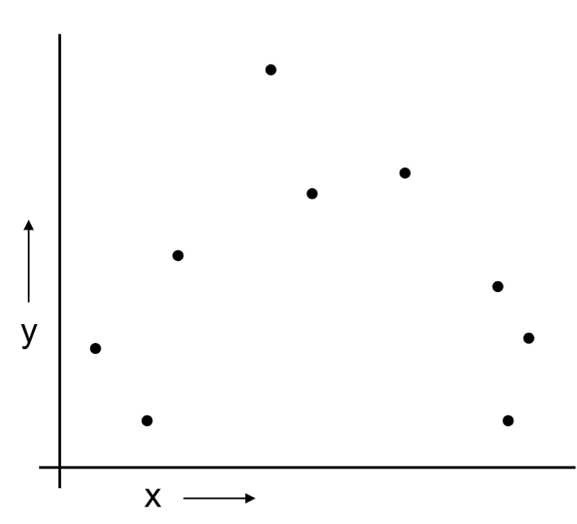
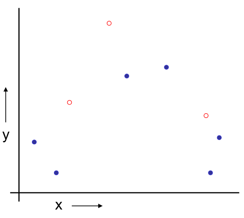
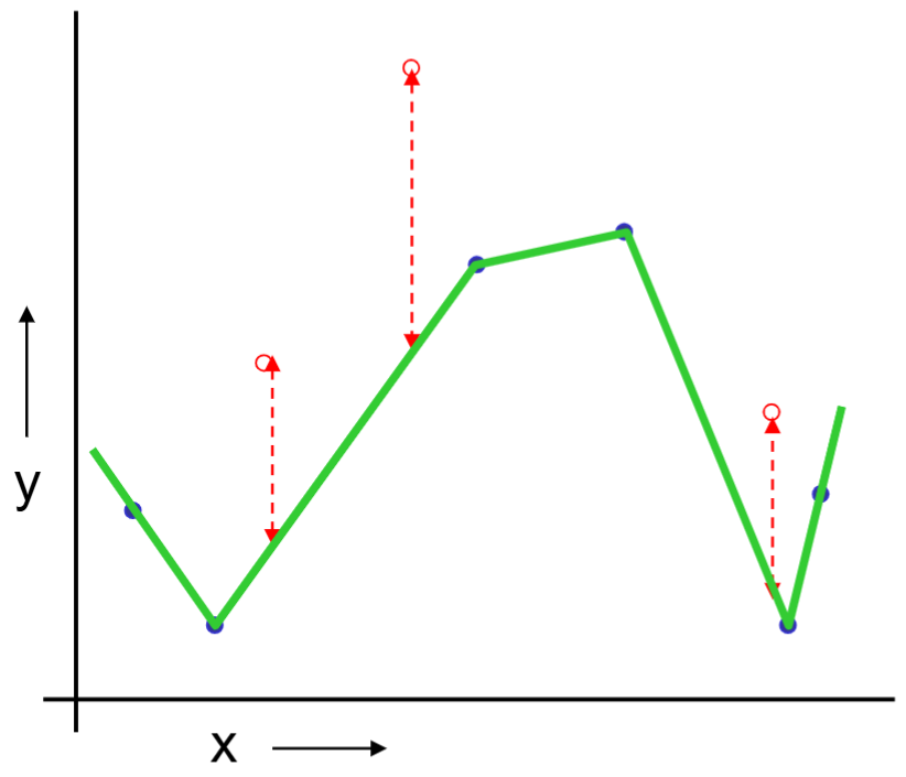
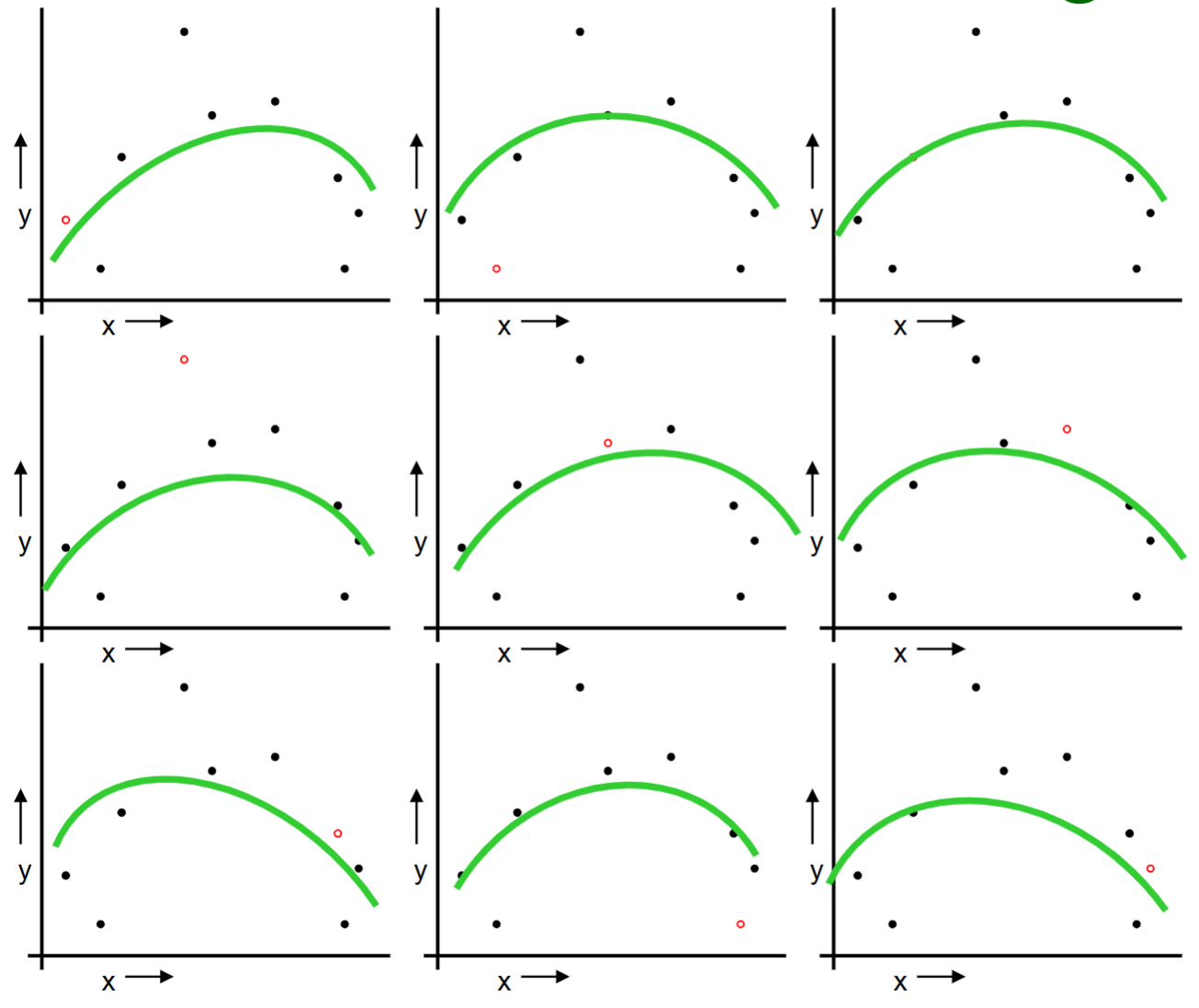
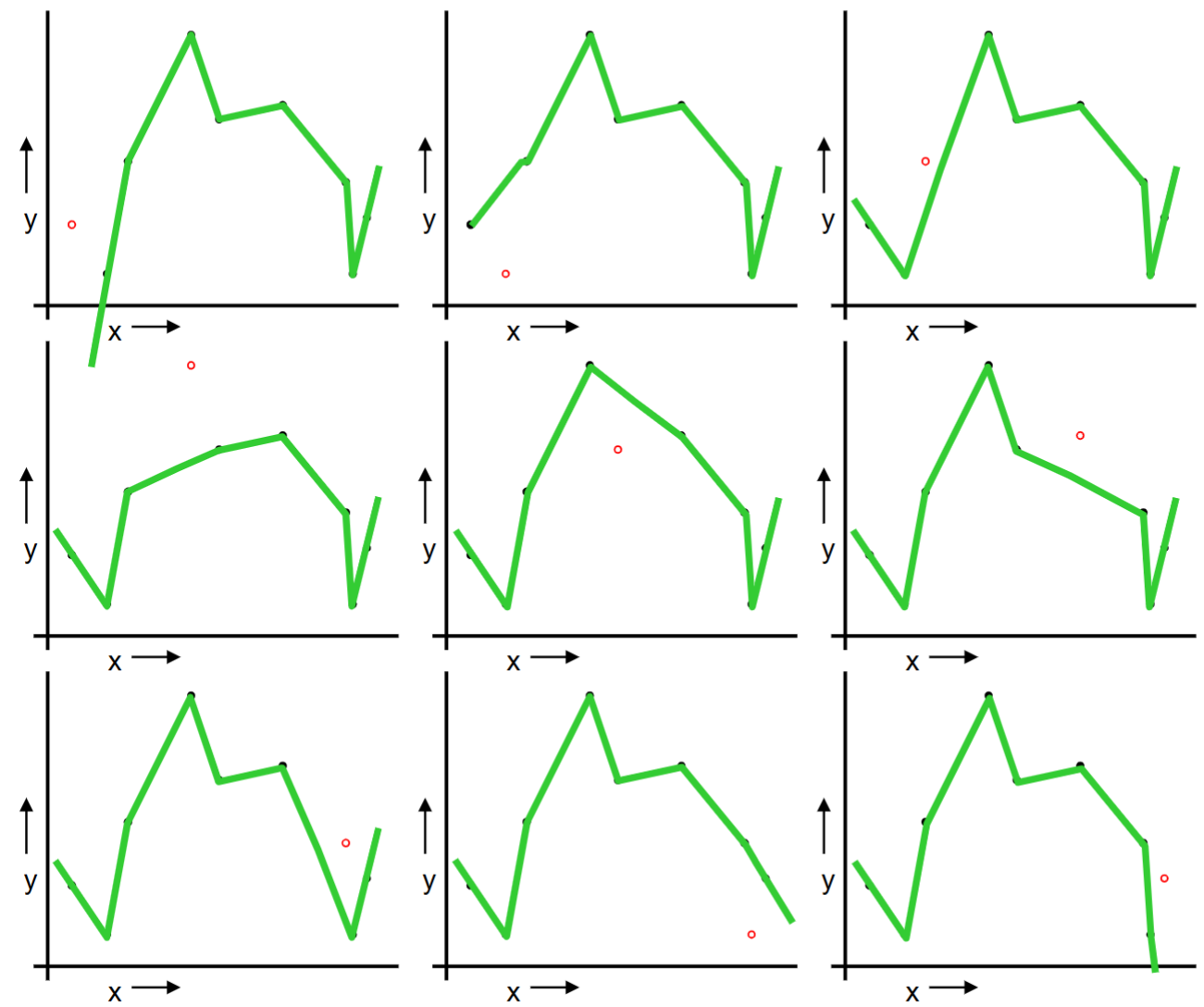
Or should we “join the dots” also know as piecewise linear nonparametric regression?
One approach to ask “How well is the model going to predict future data drawn from the same distribution?”
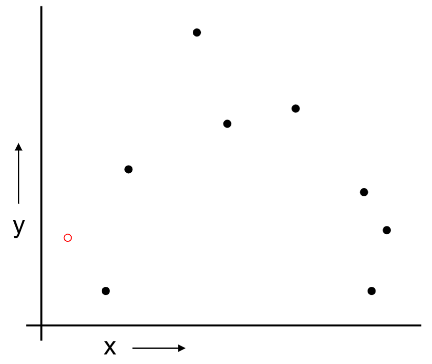
We can split the data into training and test sets. Build the model on the training set, evaluate the model on the test set.
For example, we can randomly choose 30% of the data to be in the test set and the remainder is the training set, we fit regression on the training set and estimate the model’s future performance on the test set.
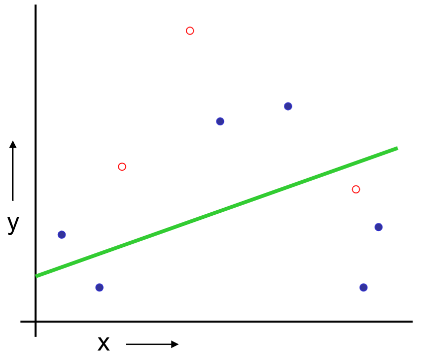
Below is an example of training and test set split.
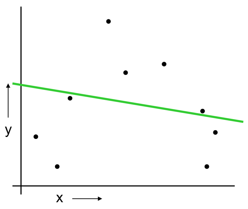
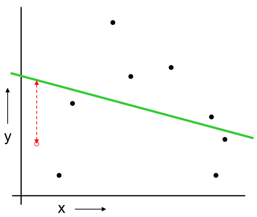
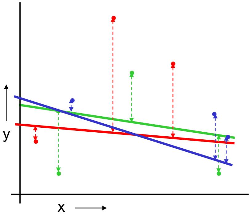
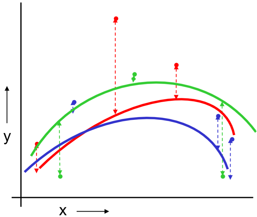
We build a linear regression on the training set.
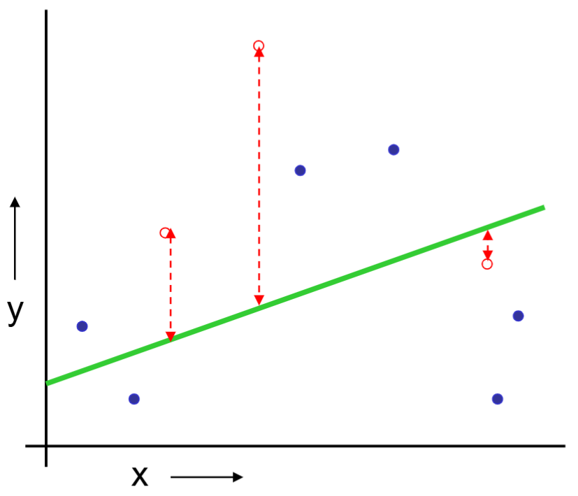
Can predict on the test set and collect the prediction errors.
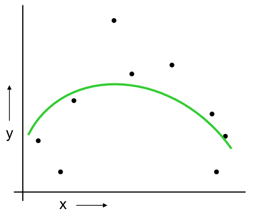
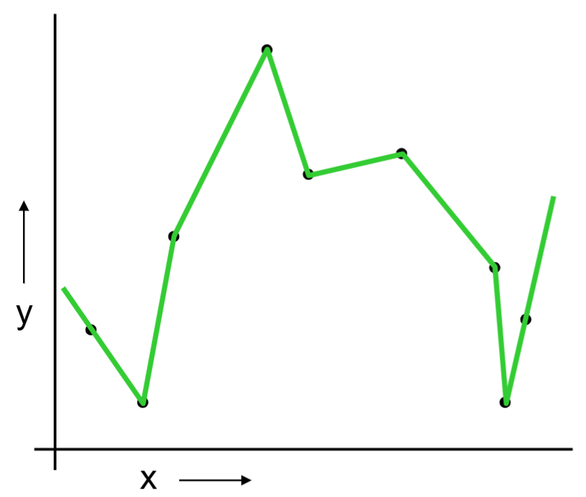
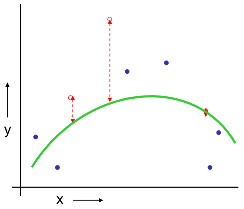
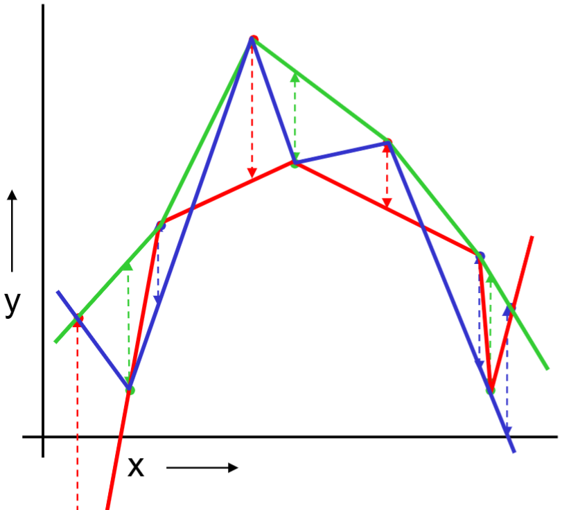
The same procedue can be done on the quadratic regression and “join the dots.”
For this training and test set split method,
The good news: very simple, just choose the model with the best test set performance.
Bad news: waste data. If we don’t have much data, our test set may be lucky or unlucky. In other words, the test set estimation of the performance is unstable.
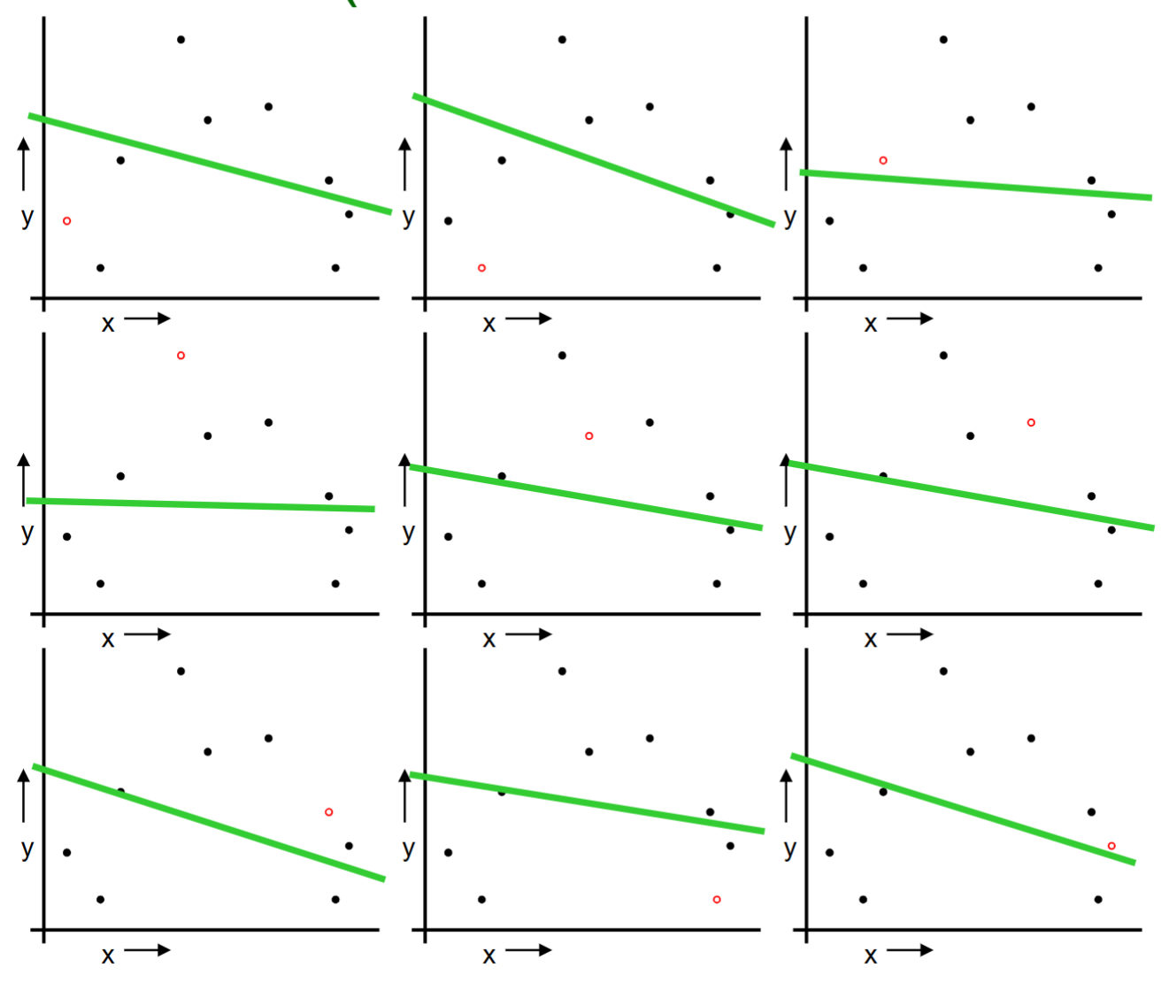
1.2. Leave One Out Cross Validation (LOOCV)
For i = 1 to n, do the following:
Temporarily remove the i-th observation (x_i, y_i) from the data.
Train the model on the remaining n-1 observations and evaluate the model on the i-th observation.
Repeat the above procedure for n times for each observation.
We can collect all the prediction errors and report the mean error.
We repeat the same procedure for quadratic regression and “join the dots.”
Let’s compare training/test split and leave one out cross validation.
Col1
Downside
Upside
Train/test split
variance: unreliable estimate of future performance
Cheap and simple
Leave one out CV
Expensive. May have some weird behavior.
Don’t waste data
Can we get the best of the both methods?
1.3. k-Fold Cross Validation
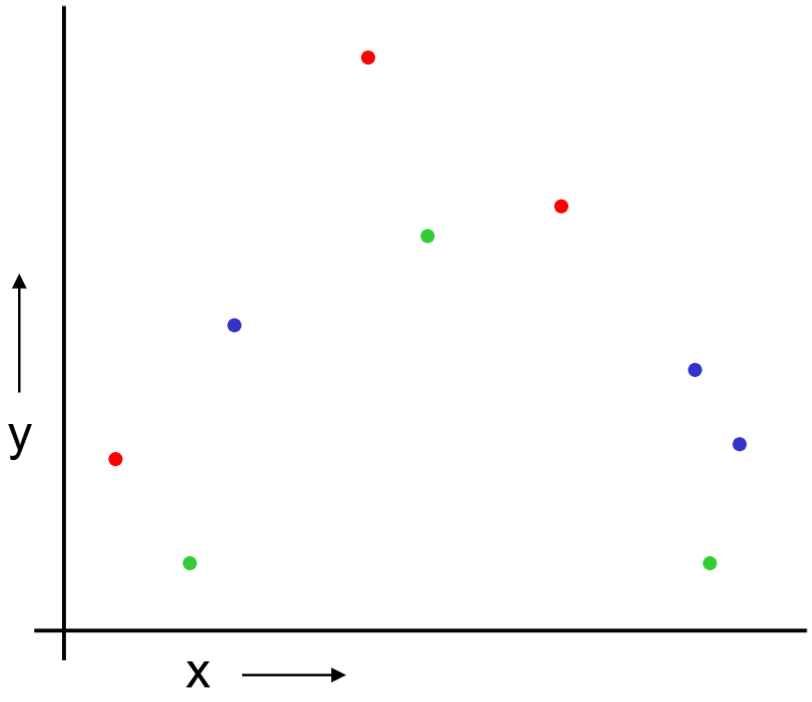
Randomly break the dataset into k partitions.
In the following example, we have k=3 partitions colored as red, green and blue.
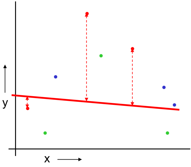
For the red partition: Train on all the points not in the red partition. Find the test-set sum of errors on the red points.
We repeat the same procedure for green and blue partitions.
We then report the mean prediction error.
Evaluation Method
Downside
Upside
Train/test split
variance: unreliable estimate of future performance
Cheap and simple
Leave one out CV
Expensive. May have some weird behavior.
Don’t waste data
10-fold CV
Wastes 10% of the data. 10x more expensive than test set
Only wastes 10%
3-fold CV
More wasted data
Slightly better than test set.
CV is used for model selection/comparison/evaluation and tuning parameter selection.
2. Evaluation of Linear Models and LASSO
2.1. Linear Models
We now use cross validation, cv.glm(), to evaluate different linear models on the Boston housing price data set. We compare the full model with the model with only two covariates, indus and rm.
The reported numbers by default are mean squared error (MSE). In its output, $delta[2] represents the bias corrected cross validation score. We can certainly change to other measure such as mean absolute deviation (MAE).
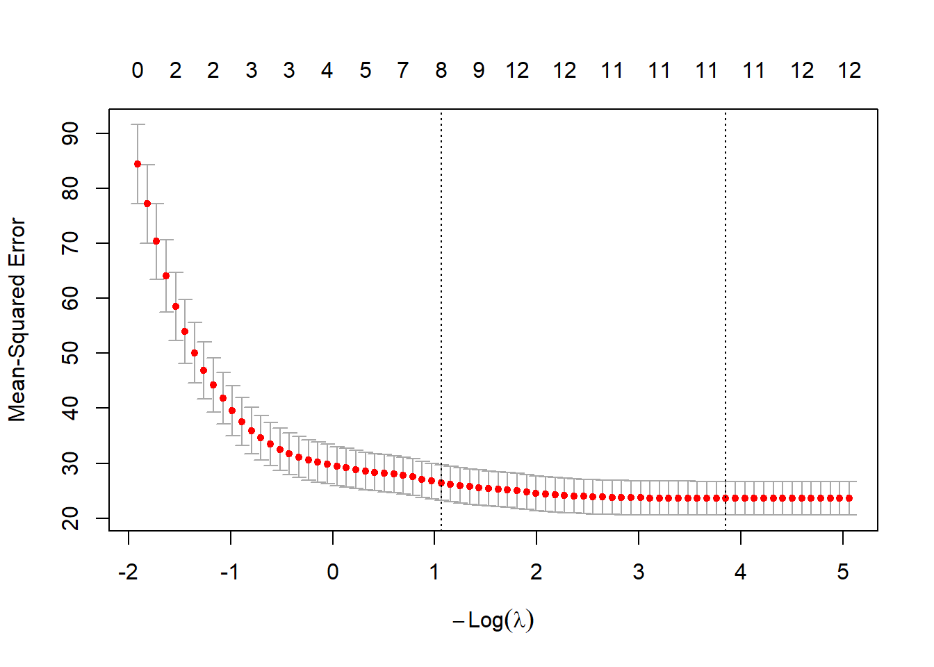
One of the most important applications of cross validation is to select the tuning parameters. For example, in LASSO, we need to select the tuning parameter \(\lambda\) which adjusts the amount of penalty on the coefficient estimate.
14 x 1 sparse Matrix of class "dgCMatrix"
             s=0.02118502
(Intercept)  34.880894915
crim         -0.100714832
zn            0.042486737
indus         .
chas          2.693903097
nox         -16.562664331
rm            3.851646315
age           .
dis          -1.419168850
rad           0.263725830
tax          -0.010286456
ptratio      -0.933927773
black         0.009089735
lstat        -0.522521473
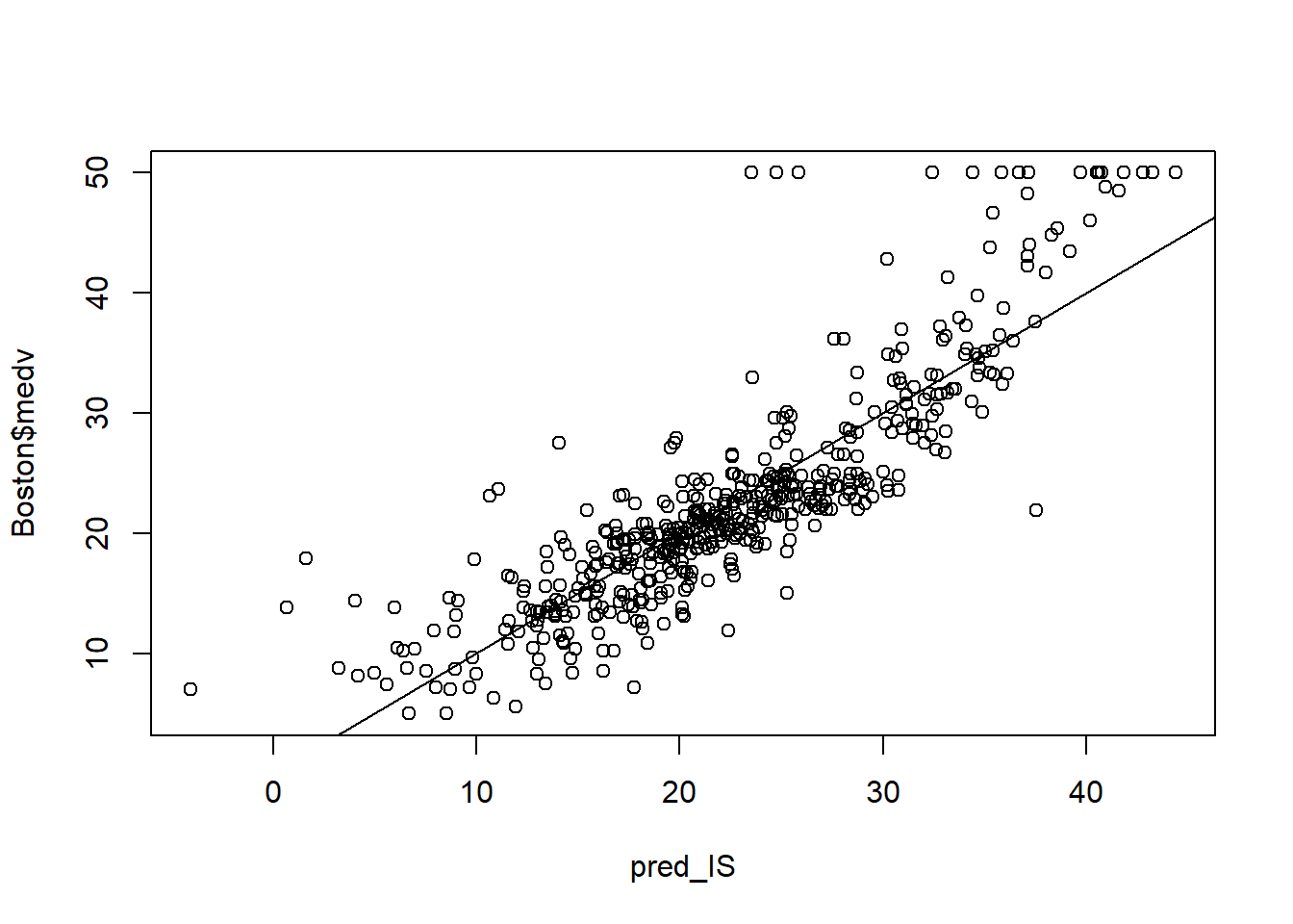
pred_IS <-predict(lasso_fit,as.matrix(Boston[, names(Boston)!='medv']),s = cv_lasso_fit$lambda.min)plot(pred_IS, Boston$medv)abline(a =0, b =1)
MSE_cost(pred_IS, Boston$medv)
[1] 21.92126
MAE_cost(pred_IS, Boston$medv)
[1] 3.259372
3. Evaluation of Logistic Regression
3.1. Evaluation Criterion
In the previous section, we focus on linear models where the response variable is numeric. To evaluate the linear models, we compare the predicted response with the actual response and obtain the prediction error, for example, MSE or MAE.
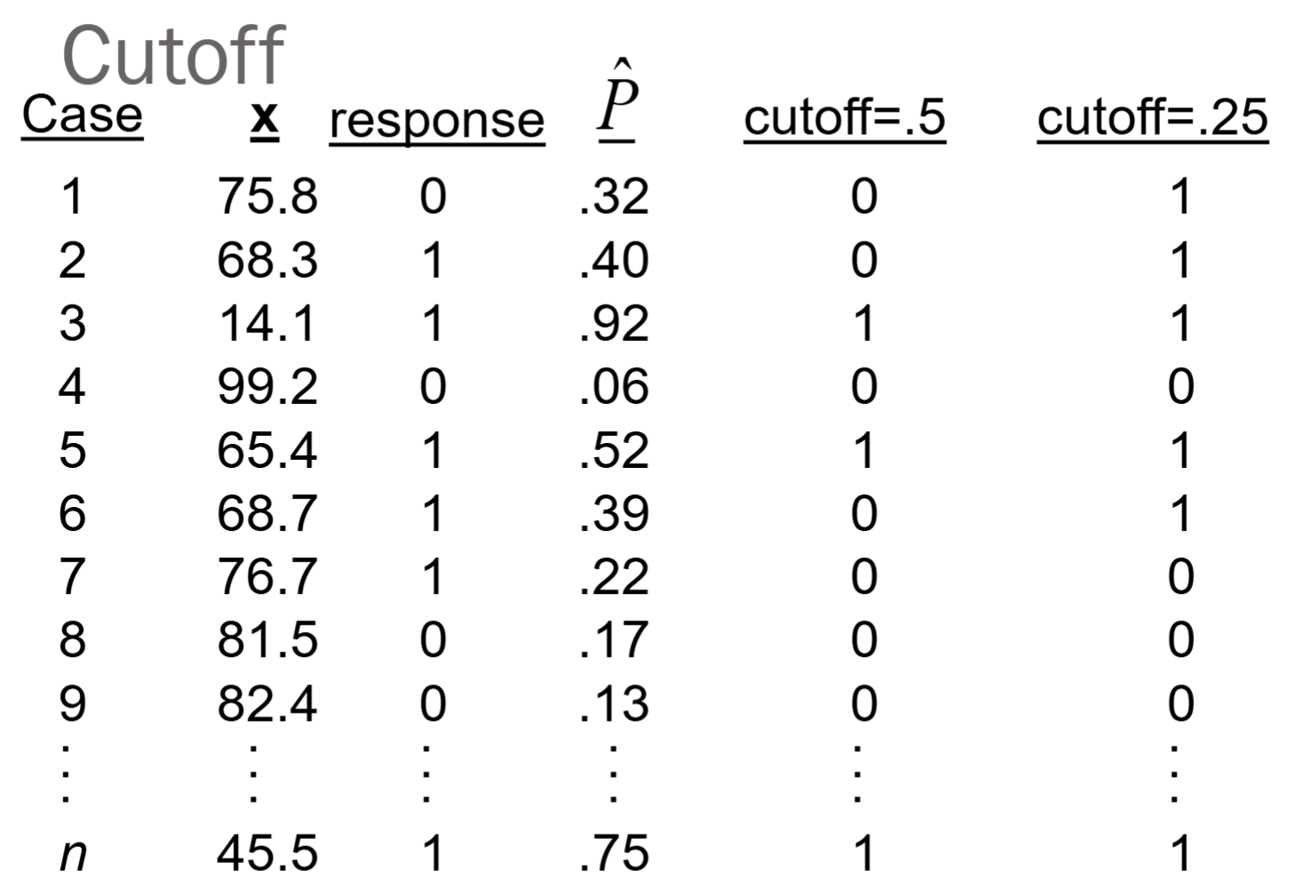
In this section, we focus on logistic regression with a binary response variable, 0 or 1. To predict the response variable using logistic regression, we need a threshold/cutoff value between 0 and 1. This is because the logistic regression provide only the probability of success at a given x.
Therefore, we can predict the response to be 0 if prob < cutoff, and predict it to be 1 if prob >= cutoff. The default cutoff is 0.5.
With the predicted response, we can compare it with the actual response using the confusion matrix below.
Confusion matrix
True label
Predicted as 0
Predicted as 1
Actual 0, negative
A, true negative
B, false positive
Actual 1, positive
C, false negative
D, true positive
The misclassification error rate = (B + C)/(A + B + C + D)
True positive fraction (TPF or sensitivity) is the proportion of positives correctly predicted as positive: D/(C+D).
False positive fraction (FPF or 1-specificity), is the proportion of negatives incorrectly predicted as positive: B/(A+B).
Note that the misclassification error rate, TPF, and FPF are all functions of the cutoff value. If we change the cutoff value, the they also changes.
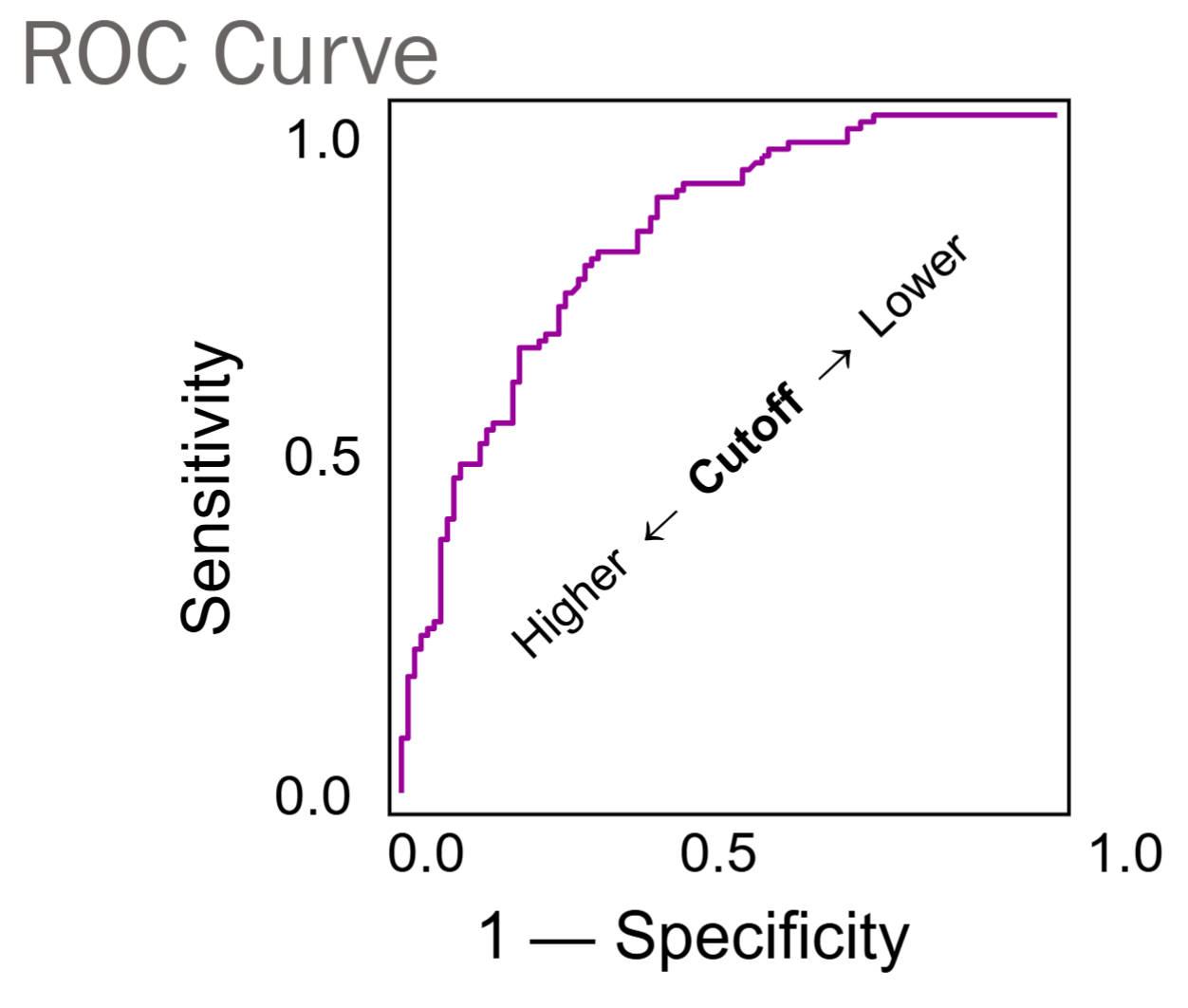
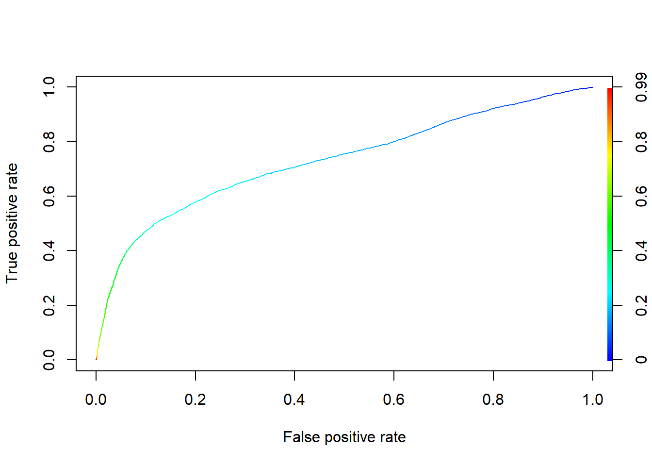
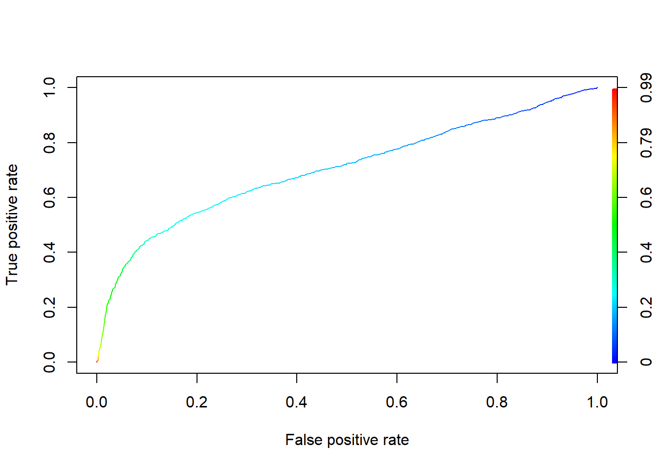
A way to expand on this idea is to get an overall measure of goodness of classification using the receiver operating characteristic (ROC) curve. ROC curve is generated by plotting FPF (1-specificity) against TPF (sensitivity) at different levels of cutoff values.
Here is an example of changing the cutoff value from 0.5 to 0.25.
If we let the cutoff value change from 0 to 1, or 1 to 0, we have the following ROC curve.
Both TPF and FPF vary inversely with the cutoff value.
The higher the cutoff, the harder it is to classify an observation as positive or 1. As the cutoff increases, both the B and D decrease.
The ROC curve shows possible TPF/FPF combinations as the cutoff value varies.
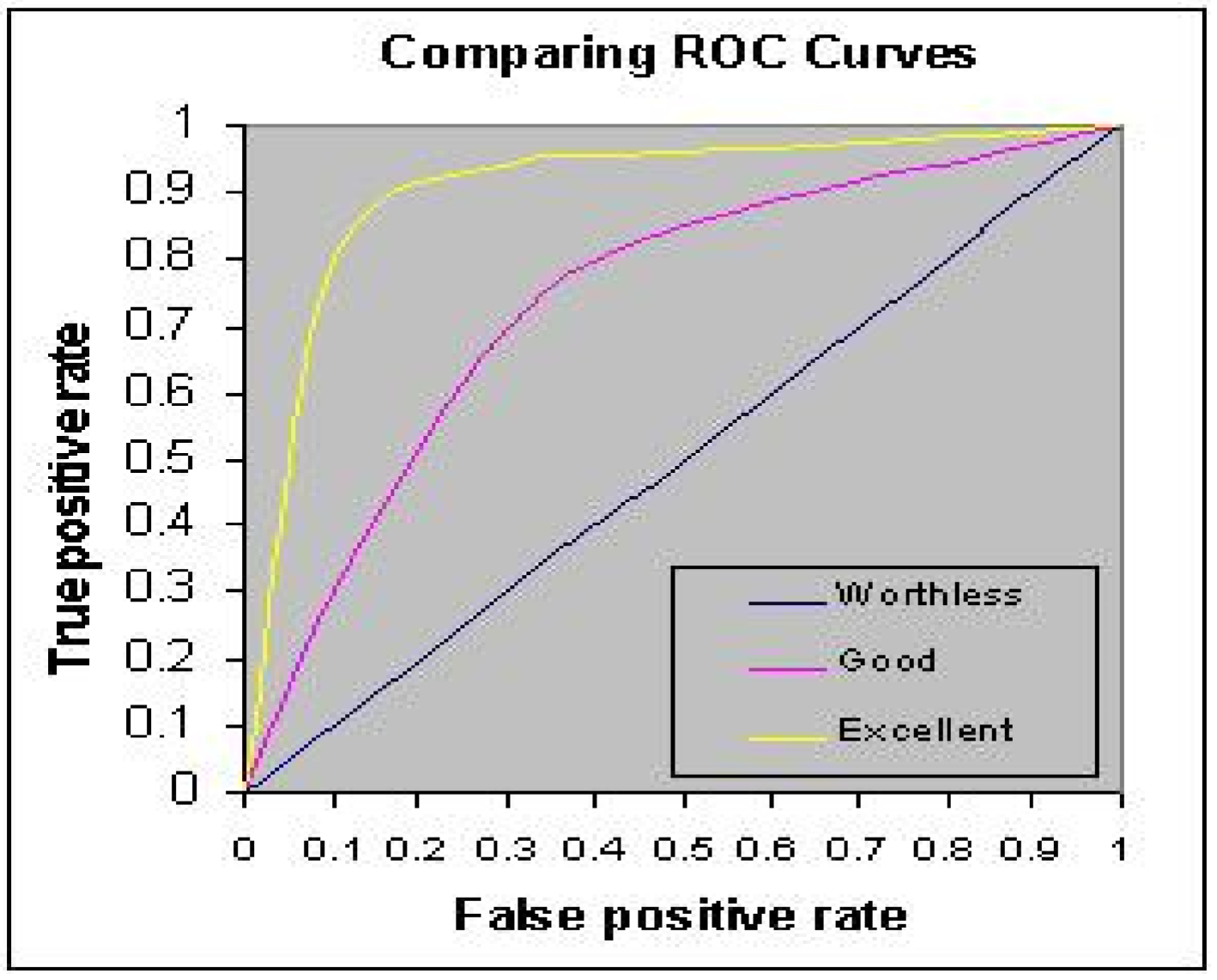
To evaluate the ROC curve, we usually use the area under the curve (AUC). A rule of thumb (industry standard) is that AUC > 0.7 represents acceptable discriminatory power.
Sometimes, we may face a slightly different binary classification problem.
For example, in bankruptcy prediction, fail to predict a bankruptcy is much more serious than predict a false bankruptcy.
Therefore, we introduce the asymmetric misclassification error rate (AMR) with a revised cutoff value pcut = 1/(1 + r)
AMR = (B + C*r)/(A + B + C + D)
Confusion matrix
True label
Predicted as 0
Predicted as 1
Actual 0, negative
A
B
Actual 1, positive
C, this is the case of Lehman Brothers
D, true positive
3.2. Training Set and Test Set Split
We use the credit data to illustrate the evaluation of logistic regression. We first split the data into training and test sets, and train the model on the training set.
Rows: 30000 Columns: 24
── Column specification ────────────────────────────────────────────────────────
Delimiter: ","
dbl (24): LIMIT_BAL, SEX, EDUCATION, MARRIAGE, AGE, PAY_0, PAY_2, PAY_3, PAY...

ℹ Use `spec()` to retrieve the full column specification for this data.
ℹ Specify the column types or set `show_col_types = FALSE` to quiet this message.
To evaluate the generalized linear model using cross validation, we use the R function cv.glm(). This function conducts the K-fold cross-validation for the generalized linear models and obtain its prediction error.
The syntax is cv.glm(data, glmfit, cost, K)
data: the full data
glmfit: the generalized linear model we build
cost: it is by default tne mean squared error (MSE) for regression. We need to adjust it for classification, e.g. ((asymmetric) misclassification rate, AUC)
K: the number of folds in cross validation. It is by default n, i.e., the sample size. Typically we use K=2, … ,10.
pcut <-0.5#Symmetric cost, equivalently pcut=1/2sym_cost <-function(r, pi, pcut=1/2){mean(((r==0)&(pi>pcut)) | ((r==1)&(pi<pcut)))}#Asymmetric cost, pcut=1/(5+1) for 5:1 ratioasym_cost <-function(obs, pred.p){# define the weight for "true=1 but pred=0" (FN) weight1 <-5# define the weight for "true=0 but pred=1" (FP) weight0 <-1 pcut <-1/(1+weight1/weight0)# logical vector for "true=1 but pred=0" (FN) c1 <- (obs==1)&(pred.p < pcut) #logical vector for "true=0 but pred=1" (FP) c0 <- (obs==0)&(pred.p >= pcut) # misclassification with weight cost <-mean(weight1*c1 + weight0*c0) # you have to return to a value when you write R functionsreturn(cost) } # end #AUC as costAUC_cost =function(obs, pred.p){ pred <-prediction(pred.p, obs) perf <-performance(pred, "tpr", "fpr") cost =unlist(slot(performance(pred, "auc"), "y.values"))return(cost)} library(boot)credit_glm <-glm(default~. , family = binomial, data = credit);
Warning: glm.fit: fitted probabilities numerically 0 or 1 occurred