BANA7046 Module 6: Classification and Regression Trees

1. Tree Models

1.1. Type of Trees

There are two type of tree models, designed for different types of response variable.

• Classification tree: response variable Y is category.

• Regression tree: response variable Y is numeric.

In this course, we have used the following data sets and its associates machine learning methods.

iris: knn, kmeans.

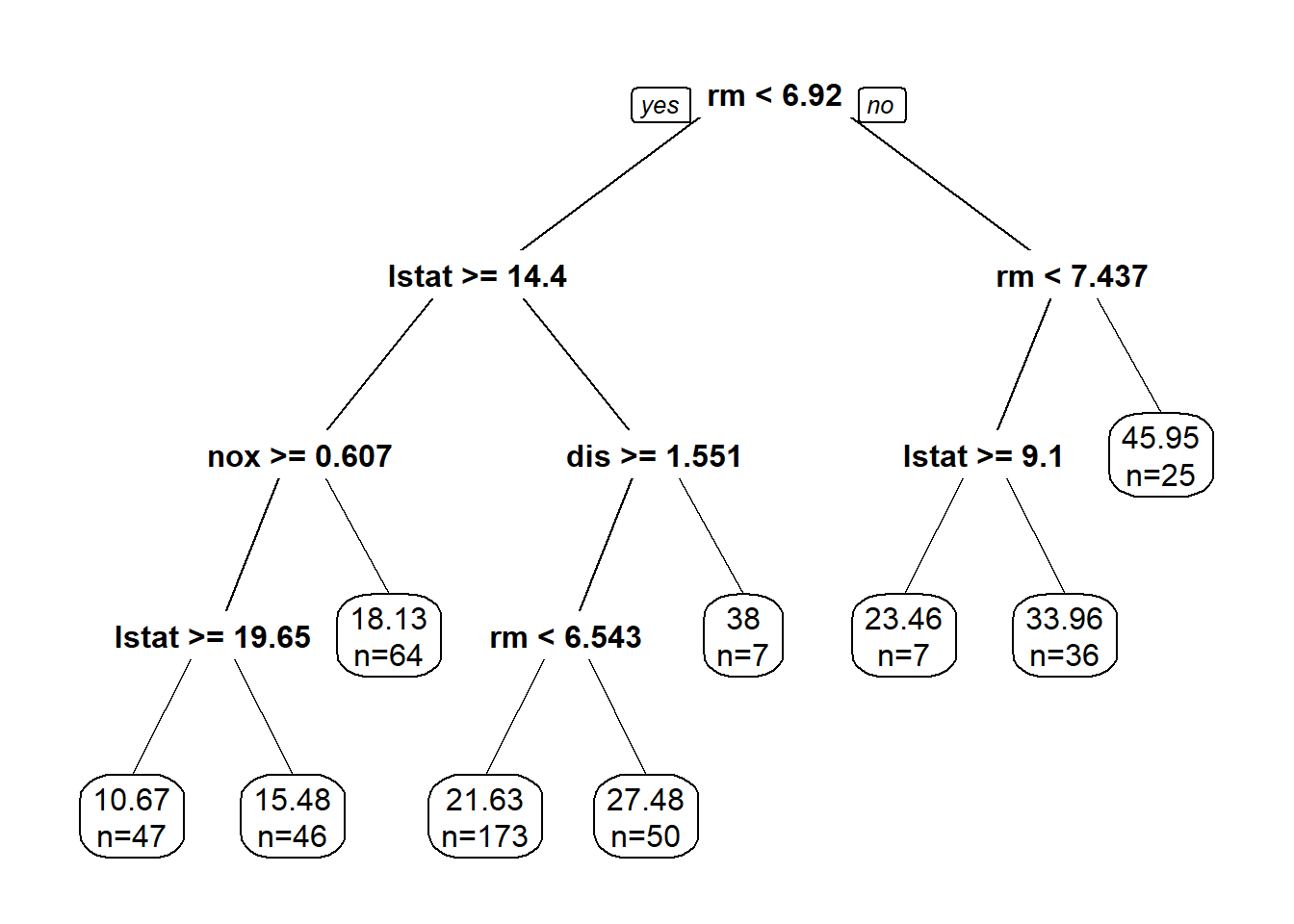
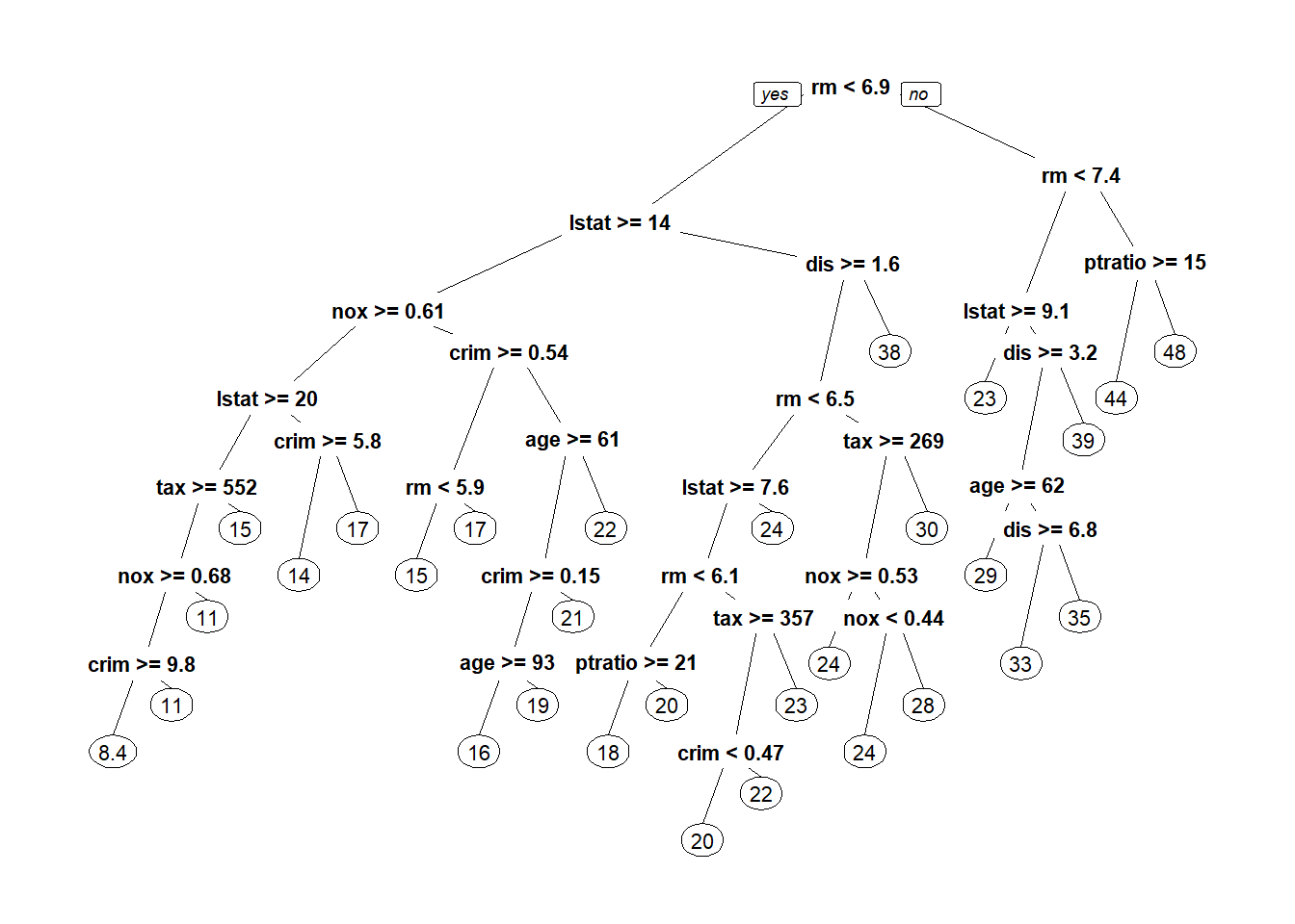
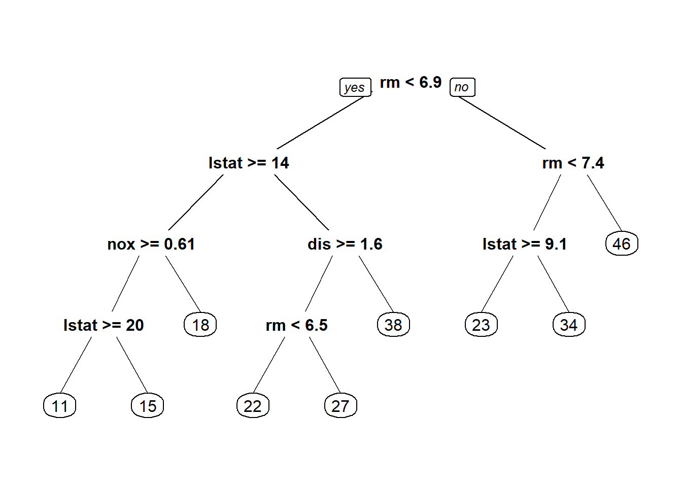
Boston housing: linear regression, LASSO, ridge regression, regression tree.

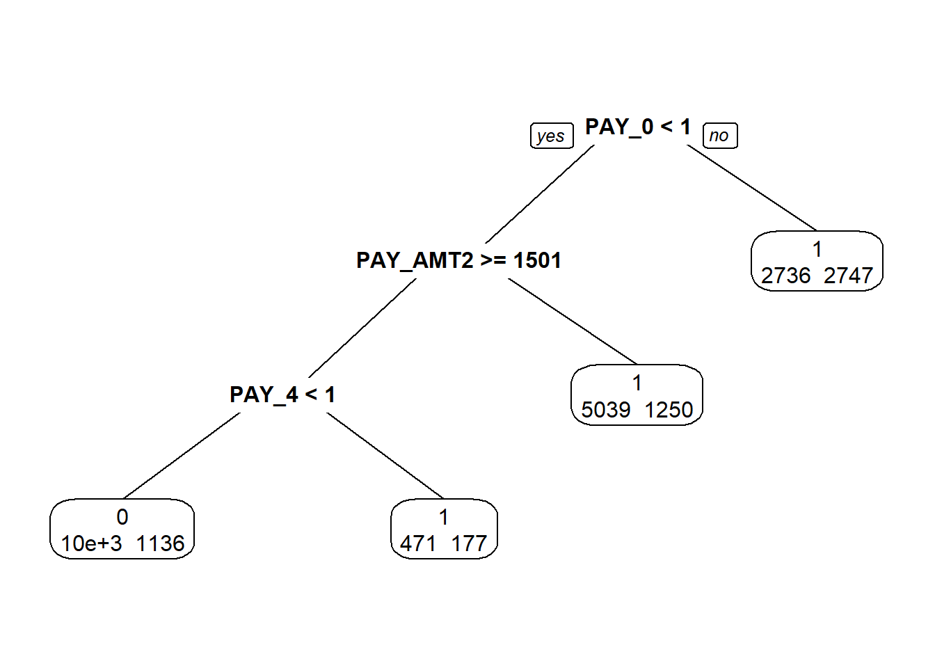
German credit, bankruptcy, credit card: logistic regression, classification tree.

1.2. Classification Trees

1.2.1. Example

Let’s look at a simple example, beer preference.

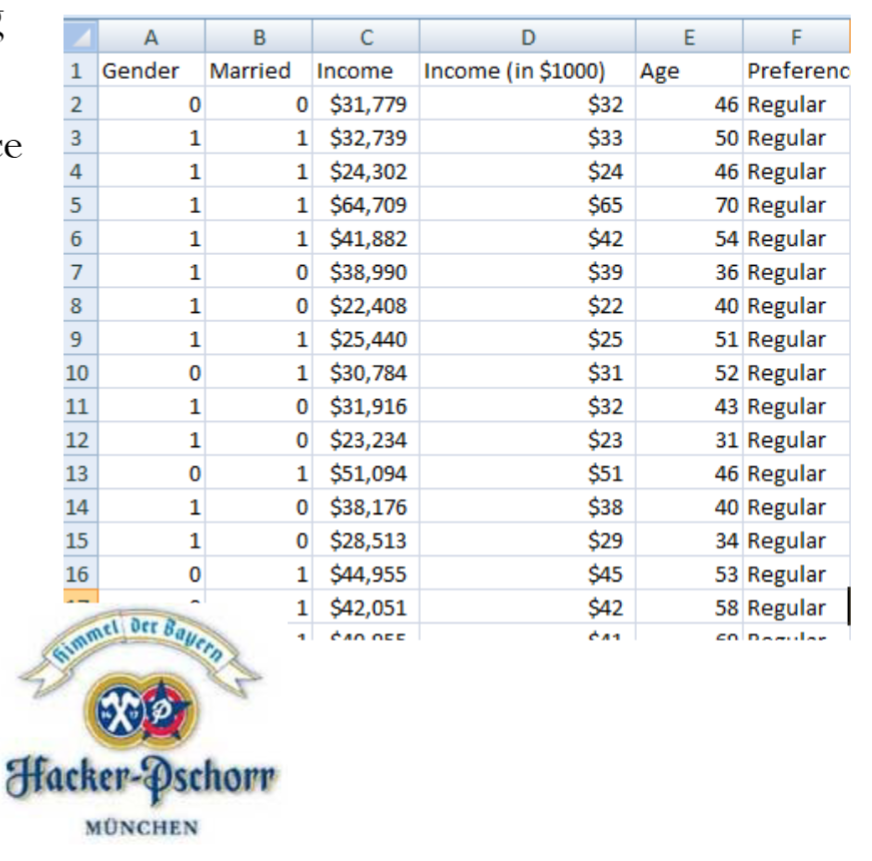
Hacker Pschorr is one of the oldest beer brewing companies in Munich. It collects data on customers’ beer preference (light/regular) and their demographic information. Its goal is to determine demographic factors for preferring light beer. For simplicity, let’s first focus on only two predictors income and age.

This is essentially a classification problem (binary: light or regular) using two predictors (income and age). Below is a snapshot of the data.

Let’s try to find the relationship between the response variable, beer preference (i.e., light/regular), and the predictors (income and age).

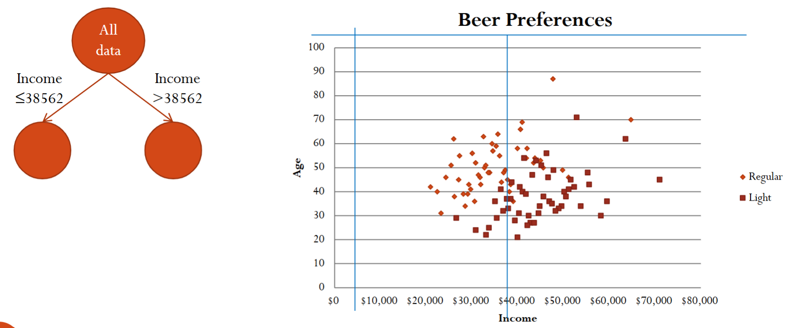
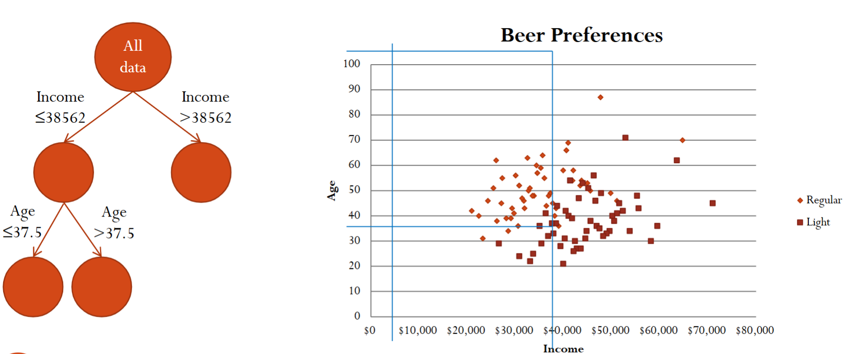
Since there are only two predictors, we can visualize the data using a scatter plot with the symbol shape representing the label.

Based on the scatterplot, we can recursively separate the records into subgroups by creating splits, i.e., thresholds, on the predictors. This splitting of the data set can be visualized as trees.

After the first split, we can further split using another predictor.

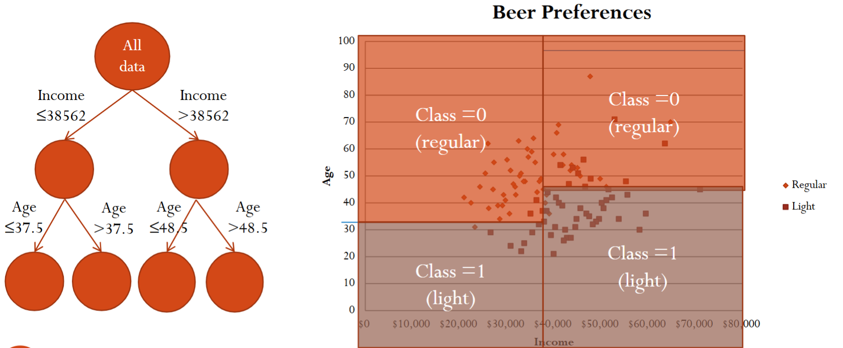
Finally, after three splits, we essentially divide the xy-plane into for different regions.

There are still some questions. For example, how to choose the split variable and its value? When should we stop growing the tree? What rule do we use for classification/prediction in the end nodes? How do we classify a new record? Below we answer these questions one by one.

1.2.2. Determining the Best Splits

What do we mean by “best”?

• We want to find the split that best discriminates between records of different classes.

• After the split we want the new sub-nodes to be more homogenous or purer than their parents nodes.

• Therefore, we need a measure of homogeneity/purity!

There are two commonly used measures for homogeneity:

• Entropy

• Gini index

Definitions are beyond the scope of this course.

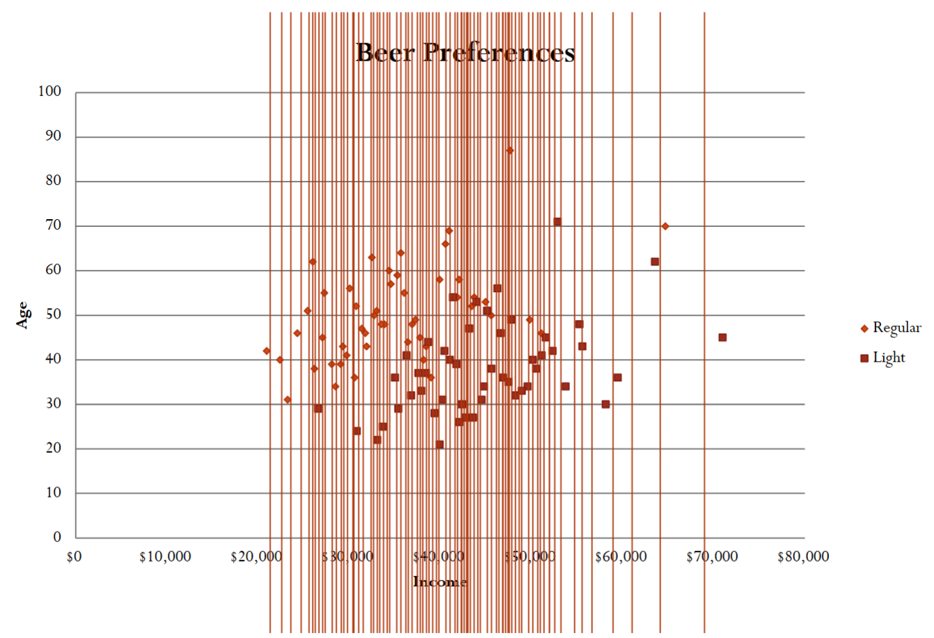
The classification and regression trees (CART) algorithm evaluates all possible binary splits.

For each variable, each possible split value is tried.

• Calculate the impurity of the resulting sub-nodes.

• Summarize the impurity of the split as the weighted average of the impurities of the sub-nodes

Select the best variable-value split.

Below is an example of searching for the best split value for the income variable.

1.2.2. When to Stop Growing Trees?

One option is to stop when we can no longer find a split that improves the impurity measures.

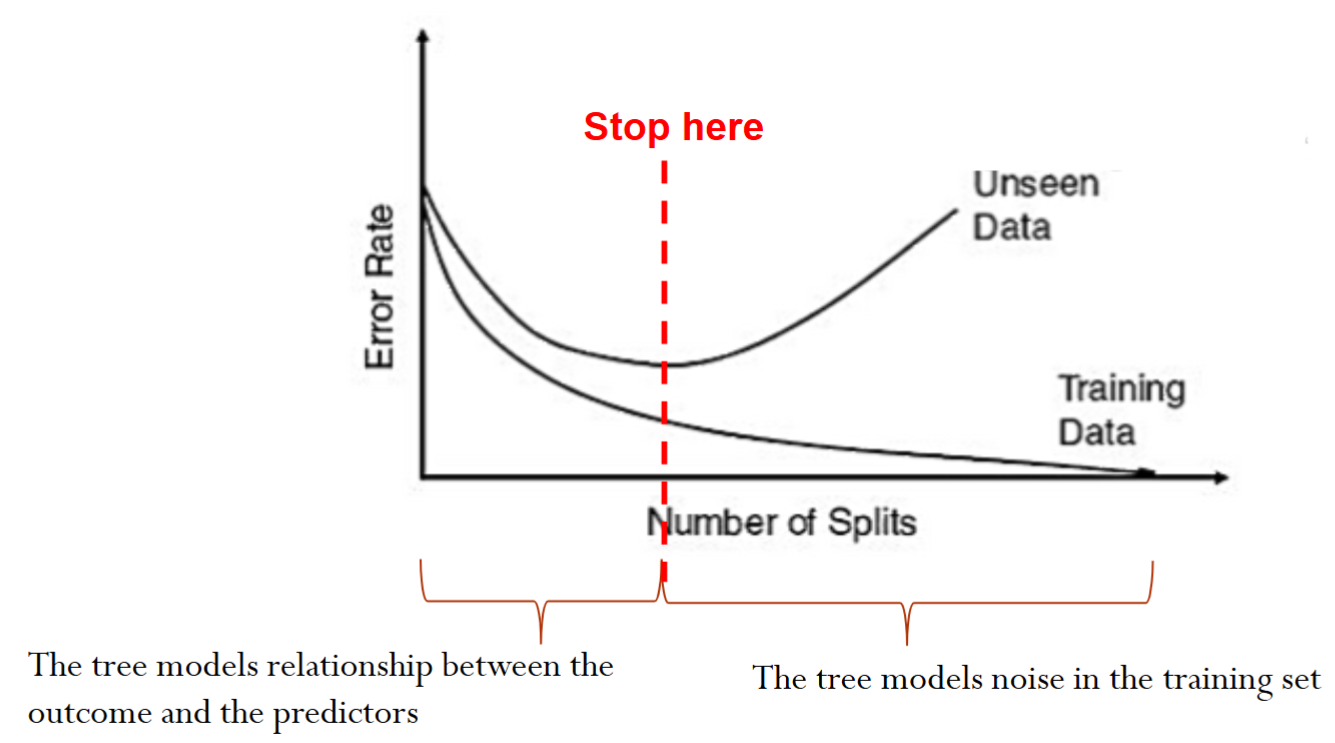
There is a chance of overfitting if we keep splitting the data until we only have very few points at each node

The goal is to arrive at a tree that captures the patterns but not the noise in the training data, therefore maximizing the prediction accuracy on new data

We can set up different stopping rules to avoid overfitting.

• Set a minimum number of records at a node.

• Set a maximum number of splits.

• Statistical significance of the split.

There is no simple good way to determine the right stopping point (depends on the dataset)

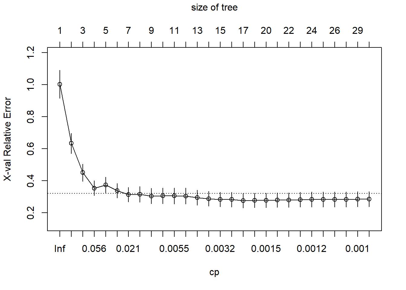
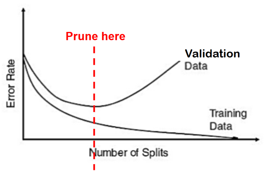
Instead of stopping rules, we can use pruning to avoid overfitting.

Pruning refers to using the validation sample to prune back (cut branches off) the full grown tree.

Pruning has been proven more successful in practice than stopping rules

Note, pruning uses the validation sample to select the best tree: the performance of the pruned tree on the validation data is not fully reflective of the performance on completely new data.

1.2.3. Prediction

To use the tree models to make prediction for a new observation, we simply need to “walk” down the tree using this observation’s predictors and find the end node that this observation falls into, and use the end node’s class to predict for this observation.

However, we need to assign a predicted class for each end node.

The default to assign a class to end node is the majority vote.

In the 2-class case: majority vote corresponds to setting the cutoff to 0.5

Changing the cutoff will change the labeling

Now, let us decide how to classify a 40 year old person with $40,000 in annual income.

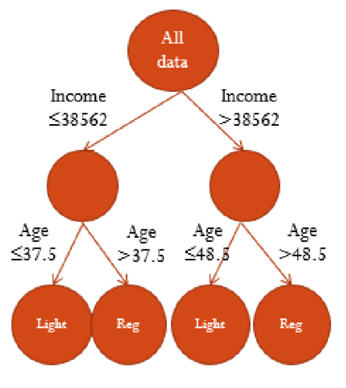
Converting a Tree into Rules

We can translate the tree into decision rules

If Income is less than or equal to $38,562 and Age <37.5 then we predict the person to like light beer.

If Income is less than or equal to $38,562 and Age is greater than 37.5 then we predict the person to prefer regular beer.

Classification and Regression Trees

Highly Interpretable

Supervised learning

Nonlinear

R: rpart (recursively partitioning trees)

1.3. Regression Tree

The regression tree is very similar to classification tree.

The only differences are

• purity measure in each node. For example, variance.

• At each end node, we need to assign a predicted value, which is often the mean of the response variable of the training observations falling into this end node.

2. Classification: Credit Card Data

2.1. Building Trees

The classification trees is slightly more complicated to specify. What makes it more complicated is that we often have asymmetric cost function. In the credit scoring case it means that false negatives (predicting 0 when truth is 1, or giving out loans that end up in default) will cost more than false positives (predicting 1 when truth is 0, rejecting loans that you should not reject).

Here we make the assumption that false negative cost 5 times of false positive. In real life the cost structure should be carefully researched.

library(rpart)
library(rpart.plot)
library(tidyverse)

── Attaching core tidyverse packages ──────────────────────── tidyverse 2.0.0 ──
✔ dplyr     1.1.4     ✔ readr     2.1.6
✔ forcats   1.0.1     ✔ stringr   1.5.2
✔ ggplot2   4.0.1     ✔ tibble    3.3.1
✔ lubridate 1.9.4     ✔ tidyr     1.3.2
✔ purrr     1.2.1     
── Conflicts ────────────────────────────────────────── tidyverse_conflicts() ──
✖ dplyr::filter() masks stats::filter()
✖ dplyr::lag()    masks stats::lag()
ℹ Use the conflicted package (<http://conflicted.r-lib.org/>) to force all conflicts to become errors

credit_data <- read_csv(file = "data/credit_default.csv")

Rows: 30000 Columns: 24
── Column specification ────────────────────────────────────────────────────────
Delimiter: ","
dbl (24): LIMIT_BAL, SEX, EDUCATION, MARRIAGE, AGE, PAY_0, PAY_2, PAY_3, PAY...

ℹ Use `spec()` to retrieve the full column specification for this data.
ℹ Specify the column types or set `show_col_types = FALSE` to quiet this message.

# convert categorical data to factor
credit_data$SEX<- as.factor(credit_data$SEX)
credit_data$EDUCATION<- as.factor(credit_data$EDUCATION)
credit_data$MARRIAGE<- as.factor(credit_data$MARRIAGE)

index <- sample(nrow(credit_data),
                nrow(credit_data)*0.80)
credit_train = credit_data[index,]
credit_test = credit_data[-index,]

credit_rpart_sym <- rpart(formula = default ~ ., 
                       data = credit_train, 
                       method = "class")
credit_rpart_sym

n= 24000 

node), split, n, loss, yval, (yprob)
      * denotes terminal node

1) root 24000 5310 0 (0.7787500 0.2212500)  
  2) PAY_0< 1.5 21490 3557 0 (0.8344812 0.1655188) *
  3) PAY_0>=1.5 2510  757 1 (0.3015936 0.6984064) *

pred_sym <- predict(credit_rpart_sym, type="class")
table(credit_train$default, 
      pred_sym, 
      dnn = c("True", "Pred"))

    Pred
True     0     1
   0 17933   757
   1  3557  1753

However, this tree with default cost minimizes the symmetric cost, which is misclassification rate. We can take a look at the confusion matrix.

credit_rpart <- rpart(formula = default ~ ., 
                      data = credit_train, 
                      method = "class", 
                      parms = list(loss=matrix(c(0,5,1,0), nrow = 2)))
credit_rpart

n= 24000 

node), split, n, loss, yval, (yprob)
      * denotes terminal node

1) root 24000 18690 1 (0.77875000 0.22125000)  
  2) PAY_0< 0.5 18517 12815 0 (0.86158665 0.13841335)  
    4) PAY_AMT2>=1500.5 12228  6565 0 (0.89262349 0.10737651)  
      8) PAY_4< 1 11580  5680 0 (0.90189983 0.09810017) *
      9) PAY_4>=1 648   471 1 (0.72685185 0.27314815) *
    5) PAY_AMT2< 1500.5 6289  5039 1 (0.80124026 0.19875974) *
  3) PAY_0>=0.5 5483  2736 1 (0.49899690 0.50100310) *

credit_rpart

n= 24000 

node), split, n, loss, yval, (yprob)
      * denotes terminal node

1) root 24000 18690 1 (0.77875000 0.22125000)  
  2) PAY_0< 0.5 18517 12815 0 (0.86158665 0.13841335)  
    4) PAY_AMT2>=1500.5 12228  6565 0 (0.89262349 0.10737651)  
      8) PAY_4< 1 11580  5680 0 (0.90189983 0.09810017) *
      9) PAY_4>=1 648   471 1 (0.72685185 0.27314815) *
    5) PAY_AMT2< 1500.5 6289  5039 1 (0.80124026 0.19875974) *
  3) PAY_0>=0.5 5483  2736 1 (0.49899690 0.50100310) *

prp(credit_rpart, extra = 1)

pred <- predict(credit_rpart, type="class")
table(credit_train$default, 
      pred, 
      dnn = c("True", "Pred"))

    Pred
True     0     1
   0 10444  8246
   1  1136  4174

The parms argument is a list. The most import element is the loss matrix. The diagonal elements are 0, and off-diagonal elements tells you the loss (cost) of classifying something wrong. For binary classification, the numbers in c() specify the cost in this sequence: c(0, False Negative, False Positive, 0). If you have symmetric cost, you can ignore the parms argument.

2.2. Prediction

There are 2 types of predictions, the probability and the actual predicted response. We use an additional argument type=“class” or type=“prob” to obtain these.

We first generate a predicted response, i.e., 0 or 1.

credit_train_pred_tree = 
  predict(credit_rpart, 
          credit_train, 
          type="class")
credit_test_pred_tree = 
  predict(credit_rpart, 
          credit_test, 
          type="class")
table(credit_train$default, 
      credit_train_pred_tree, 
      dnn=c("Truth","Predicted"))

     Predicted
Truth     0     1
    0 10444  8246
    1  1136  4174

table(credit_test$default, 
      credit_test_pred_tree, 
      dnn=c("Truth","Predicted"))

     Predicted
Truth    0    1
    0 2595 2079
    1  316 1010

We can alternatively generate the predicted probabilities, i.e., between 0 and 1.

credit_train_prob_tree = 
  predict(credit_rpart, 
          credit_test, 
          type="prob")
credit_test_prob_tree = 
  predict(credit_rpart, 
          credit_test, 
          type="prob")

cost <- function(r, phat){
  weight1 <- 5
  weight0 <- 1
  pcut <- weight0/(weight1+weight0) 
  c1 <- (r==1)&(phat<pcut) #logical vector - true if actual 1 but predict 0
  c0 <-(r==0)&(phat>pcut) #logical vector - true if actual 0 but predict 1
  return(mean(weight1*c1+weight0*c0))
}

cost(credit_train$default, 
     credit_train_prob_tree[,2])

[1] 0.9400833

cost(credit_test$default,  
     credit_test_prob_tree[,2])

[1] 0.6098333

2.3. Comparison to Logistic Regressions

#Fit logistic regression model
credit_glm <- glm(default~., 
                  data = credit_train, 
                  family=binomial)
#Get binary prediction
credit_test_prob_glm <- predict(credit_glm, 
                                credit_test, 
                                type="response")
#Calculate cost using test set
cost(credit_test$default, 
     credit_test_prob_glm)

[1] 0.6745

table(credit_test$default, 
      (credit_test_prob_glm>1/6)*1, 
      dnn=c("Truth","Predicted"))

     Predicted
Truth    0    1
    0 2107 2567
    1  296 1030

2.4. ROC and AUC

credit_rpart <- rpart(formula = default ~ .,
                      data = credit_train, 
                      method = "class",
                      parms = list(loss=matrix(c(0,5,1,0), nrow = 2)))
#Probability of getting 1
credit_test_prob_rpart = predict(credit_rpart, 
                                 credit_test, 
                                 type="prob")
#install.packages('ROCR')
library(ROCR)
pred = prediction(credit_test_prob_rpart[,2], 
                  credit_test$default)
perf = performance(pred, "tpr", "fpr")
plot(perf, colorize=TRUE)

AUC on the test set is

slot(performance(pred, "auc"), "y.values")[[1]]

[1] 0.7214135

credit_test_pred_rpart = 1*(credit_test_prob_rpart[,2] > 1/(5+1))
table(credit_test$default, 
      credit_test_pred_rpart, 
      dnn=c("Truth","Predicted"))

     Predicted
Truth    0    1
    0 2595 2079
    1  316 1010

3. Regression Tree: Boston Housing Data

3.1. Building Trees

We first load the data and create the training and test sets.

library(MASS) #this data is in MASS package

Attaching package: 'MASS'

The following object is masked from 'package:dplyr':

    select

sample_index <- sample(nrow(Boston),nrow(Boston)*0.90)
boston_train <- Boston[sample_index,]
boston_test <- Boston[-sample_index,]

The tree models are impletemented in the rpart package.

#install.packages('rpart') 
#install.packages('rpart.plot') 
library(rpart)
library(rpart.plot)
boston_rpart <- rpart(formula = medv ~ ., 
                      data = boston_train)
boston_rpart

n= 455 

node), split, n, deviance, yval
      * denotes terminal node

 1) root 455 37997.1100 22.61714  
   2) rm< 6.92 387 15548.8000 20.03902  
     4) lstat>=14.4 157  3022.6410 15.12102  
       8) nox>=0.607 93  1260.7720 13.05269  
        16) lstat>=19.645 47   417.7740 10.67234 *
        17) lstat< 19.645 46   304.5993 15.48478 *
       9) nox< 0.607 64   785.8848 18.12656 *
     5) lstat< 14.4 230  6136.7660 23.39609  
      10) dis>=1.5511 223  3167.9640 22.93767  
        20) rm< 6.543 173  1256.9280 21.62543 *
        21) rm>=6.543 50   582.4058 27.47800 *
      11) dis< 1.5511 7  1429.0200 38.00000 *
   3) rm>=6.92 68  5236.7030 37.28971  
     6) rm< 7.437 43  1819.2670 32.25349  
      12) lstat>=9.1 7   484.1971 23.45714 *
      13) lstat< 9.1 36   688.1231 33.96389 *
     7) rm>=7.437 25   450.9224 45.95200 *

prp(boston_rpart,digits = 4, extra = 1)

What is the predicted median housing price (in thousand) given following information:

crim	zn	indus	chas	nox	rm	age	dis	rad	tax	ptratio	black	lstat	medv
0.09	0	25.65	0	0.58	5.96	92.9	2.09	2	188	19.1	378.09	17.93	20.5

3.2. Prediction using Trees

We calculate the in-sample and out-of-sample prediction errors.

boston_train_pred_tree = predict(boston_rpart,
                                 boston_train)
boston_test_pred_tree = predict(boston_rpart,
                                boston_test)
mean((boston_train_pred_tree - boston_train$medv)^2)

[1] 14.06561

mean((boston_test_pred_tree - boston_test$medv)^2)

[1] 27.43894

We compare the MSE with that of linear regression below.

boston_reg = lm(medv ~ ., 
                data = boston_train)
boston_test_pred_reg = predict(boston_reg,
                               boston_test)
mean((boston_test_pred_reg - boston_test$medv)^2)

[1] 20.04389

3.3. Pruning

In rpart(), the cp (complexity parameter) argument is one of the parameters that are used to control the complexity of the tree. The help document for rpart tells you ‘’Any split that does not decrease the overall lack of fit by a factor of cp is not attempted.’’ For a regression tree, the overall R-square must increase by cp at each step. Basically, the smaller the cp value, the larger (complex) tree rpart will attempt to fit. The default value for cp is 0.01.

What happens when you have a large tree? The following tree has 27 splits.

boston_largetree <- rpart(formula = medv ~ ., 
                          data = boston_train, 
                          cp = 0.001)
prp(boston_largetree)

plotcp(boston_largetree)

You can observe from the above graph that the cross-validation error (x-val) does not always go down when the tree becomes more complex. The analogy is when you add more variables in a regression model, its ability to predict future observations not necessarily increases.

A good choice of cp for pruning is often the leftmost value for which the mean lies below the horizontal line. In the Boston housing example, you may conclude that having a tree mode with more than 10 splits is not helpful.

To look at the error vs size of tree more carefully, you can look at the following table:

printcp(boston_largetree)

Regression tree:
rpart(formula = medv ~ ., data = boston_train, cp = 0.001)

Variables actually used in tree construction:
[1] age     crim    dis     lstat   nox     ptratio rm      tax    

Root node error: 37997/455 = 83.51

n= 455 

          CP nsplit rel error  xerror     xstd
1  0.4529714      0   1.00000 1.00134 0.087657
2  0.1681547      1   0.54703 0.63290 0.063201
3  0.0780721      2   0.37887 0.45026 0.053812
4  0.0405237      3   0.30080 0.35333 0.045770
5  0.0349666      4   0.26028 0.37327 0.048376
6  0.0256857      5   0.22531 0.33746 0.045331
7  0.0170262      6   0.19963 0.31371 0.045342
8  0.0141695      7   0.18260 0.31460 0.049309
9  0.0074557      8   0.16843 0.30360 0.048236
10 0.0055721      9   0.16097 0.30537 0.049582
11 0.0054046     10   0.15540 0.30477 0.049615
12 0.0045461     11   0.15000 0.30412 0.049698
13 0.0043672     12   0.14545 0.29410 0.046345
14 0.0031674     13   0.14108 0.28724 0.045990
15 0.0031580     14   0.13792 0.28288 0.045964
16 0.0028801     15   0.13476 0.28212 0.045969
17 0.0021613     16   0.13188 0.27518 0.045602
18 0.0018053     18   0.12756 0.27661 0.045620
19 0.0013248     19   0.12575 0.27731 0.045565
20 0.0012893     20   0.12443 0.27849 0.045425
21 0.0012067     21   0.12314 0.27950 0.045419
22 0.0011849     22   0.12193 0.28166 0.046914
23 0.0011483     23   0.12075 0.28280 0.047171
24 0.0011406     24   0.11960 0.28297 0.047168
25 0.0011399     25   0.11846 0.28258 0.047171
26 0.0010270     27   0.11618 0.28306 0.047186
27 0.0010078     28   0.11515 0.28500 0.047206
28 0.0010000     29   0.11414 0.28503 0.047209

Root node error is the error when you use the sample mean for prediction. In regression case, it is the average (mean) squared error (MSE) if you use the average of medv as the prediction. Note it is the same as

mean((boston_train$medv - mean(boston_train$medv))^2)

[1] 83.51012

The first 2 columns CP and nsplit tells you how large the tree is. The rel.error × root node error gives you the in sample error.

xerror gives you the cross-validation (default is 10-fold) error. You can see that the rel error (in-sample error) is always decreasing as model is more complex, while the cross-validation error (measure of performance on future observations) is not. That is why we prune the tree to avoid overfitting the training data.

The way rpart() does it is that it uses some default control parameters to avoid fitting a large tree. The main reason for this approach is to save computation time. For example by default rpart set a cp = 0.01 and the minimum number of observations that must exist in a node to be 20. Use ?rpart.control to view these parameters. Sometimes we wish to change these parameters to see how more complex trees will perform, as we did above. If we have a larger than necessary tree, we can use prune() function and specify a new cp:

boston_pruned_tree = prune(boston_largetree, cp = 0.008)
boston_pruned_tree

n= 455 

node), split, n, deviance, yval
      * denotes terminal node

 1) root 455 37997.1100 22.61714  
   2) rm< 6.92 387 15548.8000 20.03902  
     4) lstat>=14.4 157  3022.6410 15.12102  
       8) nox>=0.607 93  1260.7720 13.05269  
        16) lstat>=19.645 47   417.7740 10.67234 *
        17) lstat< 19.645 46   304.5993 15.48478 *
       9) nox< 0.607 64   785.8848 18.12656 *
     5) lstat< 14.4 230  6136.7660 23.39609  
      10) dis>=1.5511 223  3167.9640 22.93767  
        20) rm< 6.543 173  1256.9280 21.62543 *
        21) rm>=6.543 50   582.4058 27.47800 *
      11) dis< 1.5511 7  1429.0200 38.00000 *
   3) rm>=6.92 68  5236.7030 37.28971  
     6) rm< 7.437 43  1819.2670 32.25349  
      12) lstat>=9.1 7   484.1971 23.45714 *
      13) lstat< 9.1 36   688.1231 33.96389 *
     7) rm>=7.437 25   450.9224 45.95200 *

prp(boston_pruned_tree)

Exercise: Prune a classification tree. Start with cp=0.001 and find a reasonable cp value, then obtain the pruned tree.